Antagonistic regulation for cellular intelligence

Cellular intelligence refers to information processing in single cells, i.e. genetic regulation, protein signaling and metabolic processing, all tightly integrated with each other. The goal is to uncover general ‘rules of life’ wrt e.g. the transmission of information, homeostatic and multistable regulation, learning and memory (habituation, sensitization etc.). These principles extend from unicellular organisms like bacteria to specialized cells, which are parts of a multicellular organism.

A prominent example is the ubiquitous role of feedback cycles in cellular information processing. These are often nested, or connected to a central hub, as a set of negative feedback cycles, sometimes interspersed with positive feedback cycles as well. Starting from Norbert Wiener’s work on cybernetics, we have gained a deeper understanding of this regulatory motif, and the complex modules that can be built from a multitude of these cycles by modeling as well as mathematical analysis.

Another motif that is similar in significance and ubiquity is antagonistic interaction. A prototypical antagonistic interaction consists of a signal, two pathways, one negative, one positive, and a target. The signal connects to the target by both pathways. No further parts are required.

On the face of it, this interaction seems redundant. When you connect a signal to a target by a positive and a negative connection, the amount of change is a sum of both connections, and for this, one connection should be sufficient. But this motif is actually very widespread and powerful, and there are two main aspects to this:

A. Gearshifting, scale-invariance or digitalization of input: for an input signal that can occur at different strengths, the antagonistic transmission allows to shift the signal to a lower level/gear with a limited bandwidth compared to the input range. This can also be described as scale-invariance or standardization of the input, or in the extreme case, digitalization of an analog input signal.

B. Fast onset-slow offset response curves: in this case the double transmission lines are used with a time delay. The positive interaction is fast, the negative interaction is slow. Therefore there is a fast peak response with a slower relaxation time– useful in many biological contexts, where fast reaction times are crucial.

Negative feedback cycles which can achieve similar effects by acting on the signal itself: the positive signal is counteracted by a negative input which reduces the input signal. The result is again a fast peak response followed by a downregulation to an equilibrium value. The advantage for antagonistic interactions is that the original signal is left intact, which is useful. because the same signal may act on other targets unchanged. In a feedback cycle the signal itself is consumed by the feedback interaction. The characteristic shape of the signal, fast peak response with a slower downregulation, may therefore arise from different structures.

The type of modules that can be built from both antagonistic interactions and feedback have not been explored systematically. However, one example is morphogenetic patterning, often referred to as ‘Turing patterns’, which relies on a positive feedback cycle by an activator, plus antagonistic interactions (activator/inhibitor) with a time delay for the inhibitor.

 turing_pattern

Local Adjustment of a Biochemical Reaction System

This is an explanation which refers to the paper
http://www.plosone.org/article/info%3Adoi%2F10.1371%2Fjournal.pone.0055762 (Fig.4).

Since the explanation was short at that point, here is a better way to explain it:

Image

The elementary psf results from using the kinetic parameters and executing a single reaction complex, i.e. one backward and one forward reaction. This is the minimal unit we need. For binding reactions this is A+B <->AB (forward kon, backward koff), for enzymatic reactions it is  A+E<->AE->A* and A*->A.(forward kon, backward koff, kcat and kcatd)

But in a system, every reaction is embedded. Therefore the elementary psf is changed. Example:
one species participates in two reactions and binds to two partners. The kinetic rate parameters for the binding reaction is the same, but some amount of the species is sucked up by the other reaction.
Therefore, if we look at the psf, its curve will be different, and we call this the systemic psf. It obviously depends on the collection of reactions, as a matter of fact on the collection of ALL connected reactions, what this psf will look like.

Now in practice, only a limited amount of “neighboring reactions” will have an effect. This has also been determined by other papers, i.e. the observation that local changes at one spot do not “travel” far.
Therefore we can now do a neat trick:

We look at a whole system, and focus in on a single psf, which means a systemic psf. Example:
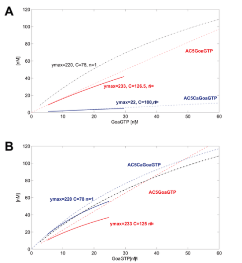
GoaGTPO binds to AC5Ca and produces GoaGTPAC5Ca. In this system, the binding reaction is very weak. The curve over the range of GoaGTP (~10-30nM) goes from near 0 to maybe 5 nM at most. We may decide or have measured that we want to improve the model at this point. We may use data that indicate a curve going from about 10nM to about 50nM for the same input of GoaGTP (~10-30nM). Good thing is that we can define just such a curve using hyperbolic parameters. We have measured or want to place the curve such that ymax=220, and C=78, n=1.

So now we know what the systemic psf should be, but how do we get there? We adjust the underlying  kinetic rate parameters for this reaction and any neighboring reactions such that this systemic psf results (and the others do not change or very little).
This can  obviously be done by an iterative process

  • adjust the reaction itself first, (change kinetic rates)
  • then adjust every other reaction which has changed,(change kinetic rates)
  • and continue until the new goal is met and all other psfs are still the same.
  • Use reasonable error ranges to define “goal is met” and “psfs are the same”.

Without error ranges, I do not offer a proof that such a procedure will always converge. As a matter of fact I suspect it  may NOT always be possible. Therefore we need reasonable error ranges.
In practice, in most cases I believe 2,3, maybe 4 reactions are all that is affected, everything else will have such small adjustments that it is not worth touching. These functions remain very local. In the example given, only one other reaction was changed at all.

The decisive part is that we can often measure such a systemic psf, such a transfer function somewhere in the system, and therefore independently calibrate the system.

We measure the systemic psf, but we now have a procedure to force the system into matching this new measurement by adjusting kinetic rates, and using the psf parameters to define the intended, adjusted local transfer function.

In many cases, as in the given example, this allows to locally and specifically test and improve the system – this is novel, and it only works because we made the clear conceptual difference between kinetic rate parameters (which are elementary) and systemic psf parameters.

We do not derive kon vs. koff or the precise dynamics in this way.  For a binding reaction it is only the ratio koff/kon (=Kd) that matters, for an enzymatic reaction it is koff/kon and kcat/kcatd. There are multiple solutions. Dynamic matching may filter out which ones match not only the transfer function, but also the timing. This has not been addressed, because it would only be another filtering step.

The procedure outlined for local adjustment of a biochemical reaction system needs to be  implemented,and more experience gained on spread of local adjustments and reasonable error bounds.